Boolean and Gene Regulatory Networks

Requires a Wolfram Notebook System
Interact on desktop, mobile and cloud with the free Wolfram Player or other Wolfram Language products.
Boolean networks have a wide range of applicability, including the modeling of systems regulating the actions of genes and the proteins they produce [1, 2]. Such networks are characterized by different cycles of states and corresponding basins of attraction (i.e. the sets of states that evolve into given cycles) and comprise what is generally known as a state machine [3]. Those networks are found to be generally analogous to different types of biological cells, including both normal and cancerous ones. Therefore, it is useful to be able to understand and design such networks for robustness and controllability [4]. This program seeks to illustrate different networks, the cycles or attractors they produce, and how they depend on the selection of different rules that govern individual bits in the state machine.
Contributed by: Jim Wiggins (August 2018)
Based on a program by: Garett Neske
Open content licensed under CC BY-NC-SA
Details
Overview
Boolean networks are described in terms of the number of bits  composing them and in terms of the number of inputs
  to each of the logic gates or rules that control each of their transitions from a current state to the next state. Binary weighting of those bits gives a numerical value to each possible state for the entire system. The display will generally show graphically the transitions from one state to the other, along with the cycles the networks may consist of.
Refer to the numbered snapshots in the Snapshot section in the notebook file or select the corresponding Bookmark in the CDF application.
Controls
The display is organized into a central area for graphs and text characterizing different networks, along with five rows of controls to select and display different operating features and aspects of each network.
Bits (N), Rule inputs (K) and Rules and sources
Use "Bits (N)" to select the number of bits in a system, which can be 8, 10, 12, 14 or 16, to determine the range and number of state values in the system. For example, with 12 bits selected, the possible set of states will range from 0 to 4095 inclusive. The genes or bits are binary weighted with bit 1 being the most significant and bit 12 being the least significant.
Use "Rule inputs (K)" to select 2, 3 or 4 bits as sources to control the operation of each bit.
Use "Rules and sources" to select, with  , from four sets of preset rules (1, 2, 3, 4) and rule inputs, or from a "Random" selection of them. With
  or
or  , only the "Random" selection is possible; clicking the numbers 1 through 4 will generate a beep and a new random selection.
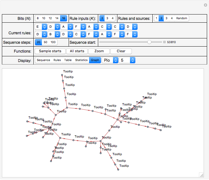
Snapshot 1, with "Display" set to "Rules", shows a system with 12 bits, three inputs for each of the 12 bits and a more or less random selection from a set of six logical rules that are indicated in the "Current rules" set of controls. Rules "A" through "F" correspond to and select from a standard set of logic functions (AND, NAND, XOR, XNOR, NOR and OR) for each bit.
Also shown in the display area of Snapshot 1 is information that, for example, the next state of bit 1 (top left) will be determined by the operation of RuleK3F (OR) and by the current states of inputs from bits 5, 7 and 9.
Current rules
Use each of the  popup menu controls to select from the set of six possible logic functions for each bit. This will generally affect the sequential evolution of the states in the network and the size and number of cycles in it.
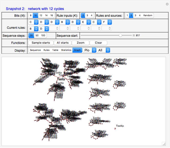
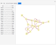
For example, Snapshots 2 and 3, with "Display" set to "Graph," show the effects of changing the rule for bit 2 from "D" to "A"; that is, the number of cycles in the system has changed from 12 to 6.
Sequence steps and Sequence start
Generally, the program applies the different sets of logic rules to the current state to generate a next state for a specified number of steps determined by the "Sequence steps" control. Use the "Sequence start" slider to select a new starting state for the sequence. Multiple starts are stitched together to provide various pictures—with the use of the "Graph" option of the "Display" control—of the entire network.
Snapshot 4, with the "Display" type set to "Sequence," shows a progression of the network states for the number of steps equal to different settings of the "Sequence steps" control, in this case, 20. Generally, most systems evolve into cycles (attractors) within 20 steps, so selecting more than that is typically an unnecessary waste of processing time. For example, in Snapshot 4 the cycle is {13741, 7657, 12717, 7609, 429, 7608, 1453, 7656, 13741}, which repeats several times up to the limit set by "Sequence steps."
Functions: Sample starts, All starts, Zoom, Clear
This row provides a general set of functions to generate sets of sample sequences, to enlarge graphical displays and to clear the collection of sequences.
Click "Sample starts" to generate a random selection of sequences, 20 for  , 50 for
  and 100 for
  . Snapshot 5, with "Display" set to "Statistics" shows, in the "Coverage" item, that 212 states have been evaluated in the state sequence evolution. Also shown is that the sequence generation has produced five cycles, two singletons, a doubleton and two cycles of four.
Click "All starts" to generate sequences starting from the full set of possible states, for example, 1024 for  . Note this feature is only available for
  as it is too time-consuming to generate the full set of sequences in other cases. While the sequence starts are being evaluated, the "All starts" button will remain in the pressed state—typically about three seconds for
  . When this is done, the "Coverage" line will show that all states in the set of possibilities (0 to 1023) have been evaluated.
Click "Zoom" to change the magnification factor for the plotting of cycles and basins of attraction; see Snapshot 6 for a single plot from a set of 12. Note that placing the tooltip over a state (blue dots) will show the state values.
Click "Clear" to more or less clear the collection of sequences; the only one remaining in the list is the one corresponding to the last sequence start evaluated.
Display: Sequence, Rules, Table, Statistics, Graph
This row provides a set of functions to display different features and aspects of the system being evaluated.
Click "Sequence" to see the last sequence generated. This is typically used to see the effects of changing the "Sequence start" control (see Snapshot 4).
Click "Rules" to see the sets of rules that govern the evolution of system states, and the sets of inputs on which they depend. See Snapshot 1 for an example. Rules are in decreasing weight—relative to the state values—from left to right and from top to bottom in that snapshot and correspond to the set of  rule selectors in the "Current rules" rows.
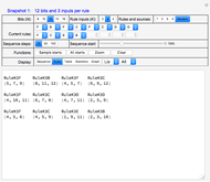
Click "Table" to see the truth tables for the outputs of the six possible logic functions—"A" through "F"—for each of the  inputs (see Snapshot 7).
Click "Statistics" to see the number of cycles and the states that comprise them. Snapshot 8 shows 12 cycles (two cycles of three states each, one singleton cycle and nine cycles of seven states each). Each cycle begins and ends with the same value for display purposes.
Click "Graph" to display different types and formats and sets of sequence data selected by the two controls to the right of it. Generally, what is shown in the following variations associated with "Graph"—items 1 to 4 following—are the different cycles and the tributaries leading to them, either "All" of them or individually:
1. Select "List" to see either a list of all cycles or a single one, each sublist starting with the cycle found ("None" if there is not one)—indicated by the first and last values being equal, along with all of the tributaries leading to the individual cycle. The tributary sequences end in a state that is part of the indicated cycle. For instance, Snapshot 9 shows the full set of cycles, the first of which is a cycle of length 3 (37, 471, 879), along with a set of tributary sequences for that cycle, the second of which is {823, 429, 198, 878, 39, 454, 879}.
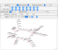
2. Select "Plot" to show a graphical representation of the sequences and cycles; see Snapshot 6 (with "Zoom" set to 2) for an individual plot and Snapshot 2 for the full set ("All").
3. Select "Array" for an array plot representation of the cycles, either individually or all of them. See Snapshot 10 for the latter. Note that this display clearly indicates which bits do not change over the course of the cycle and which ones do.
4. Select "Bits" to see the binary representations of the cycle(s) selected by the rightmost control.
Sometimes and for some networks, the system does not find all the cycles that are actually present. Snapshot 11 corresponds to a network with a different set of "Rules and sources" and, with "Sequence steps" set to 20, the system finds only two different cycles, the first of which is "None" as indicated in the "Statistics" display. And a display of that cycle with "Graph", "Plot" and "1" (not shown) will show that many of the tributaries have been stitched together into what are apparently, though not actually, several different cycles.
See Snapshot 12, which corresponds to the same network as in Snapshot 11, but with "Sequence steps" set to 50—normally, you would select "Clear" and then "Sample starts" to generate the data shown. The display of the "Statistics" for the network shows the network to possess one of the same cycles as those in Snapshot 11; that is, {99, 297 ... 99}, along with eight additional ones, each of which consists of 30 states.
References
[1] S. B. Cahn and S. G. J. Mochrie, "Biologic: Gene Circuits and Feedback in an Introductory Physics Sequence for Biology and Premedical Students." arxiv.org/abs/1307.3126.
[2] Wikipedia. "Gene Regulatory Network." (Jul 27, 2018) en.wikipedia.org/wiki/Gene_regulatory_network.
[3] Wikipedia. "Finite-State Machine." (Jul 27, 2018) en.wikipedia.org/wiki/Finite-state_machine.
[4] Y. Xiao, "A Tutorial on Analysis and Simulation of Boolean Gene Regulatory Network Models," Current Genomics, 10(7), 2009 pp. 511–525. doi:10.2174/138920209789208237.
Snapshots


Permanent Citation
 Elementary Cellular Automaton with Network
Francis A. Bitonti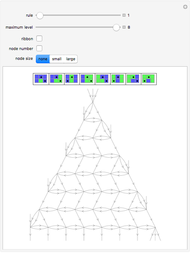 Causal Network Generated by a Mobile Automaton
Abigail Nussey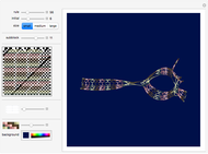 Automata Generative Networks 2
Kovas Boguta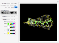 Automata Generative Networks 1
Kovas Boguta Cellular Automata on Trivalent Networks
Seth J. Chandler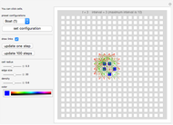 Network View of Conway's Game of Life
Yoshihiko Kayama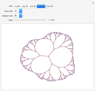 Planar Three-Connected Trivalent Network Mobile Automaton
Tommaso Bolognesi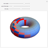 Cellular-Automaton-Like Neural Network in a Toroidal Vector Field
Benjamin I. Rapoport Cellular Automaton Browser
Jim Gerdy Cellular Automaton Rules on Dendrites
Jim Gerdy