Boundary Value Problems for Cone Geodesics

Requires a Wolfram Notebook System
Interact on desktop, mobile and cloud with the free Wolfram Player or other Wolfram Language products.
Geodesics are an important concept in differential geometry. Roughly speaking, a geodesic is locally the shortest path joining two points on a surface. However, extending a geodesic does not necessarily give the shortest path between two endpoints. For example, on a sphere the geodesics are arcs of great circles, which are the unique shortest paths between their endpoints only when the arc is smaller than a semicircle.
[more]
Contributed by: Raja Kountanya (April 2014)
Open content licensed under CC BY-NC-SA
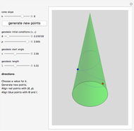
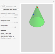
Snapshots


Details
The geodesic curve connecting two points on a surface of revolution as a boundary value problem (BVP) can be solved through the Euler–Lagrange (EL) equations [1]. A geodesic starting in a certain direction from a given point on the surface is an initial value problem (IVP) and can be solved through the canonical geodesic (CG) equations [2]. A marching scheme for the latter has been implemented for a torus [3] and hyperboloid [4].
For a cone [5] and pseudosphere [6], intrinsic properties of geodesics were used that can be generalized to find the geodesic connecting two points on the respective surfaces. However, for engineering applications, it is useful to know the construction from the ground up so that the method can be used for other general surfaces of revolution as, for example, in the many shapes encountered in manufacturing science.
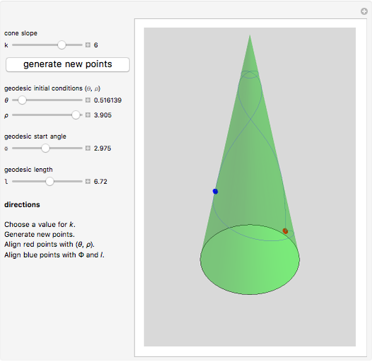
This Demonstration takes up the surface of a cone again and shows the construction of a geodesic as both a BVP and an IVP. Taking two random points on the surface, the BVP curve joining the two points is plotted. With the right initial conditions, the IVP can be made to coincide with the BVP. Moreover, when the cone taper angle is small enough, multiple geodesics can be made to pass between the two points.
Consider a cone where the origin is set to the apex and the positive  axis points to the base. It can be parameterized with radius
  and angle θ, the latter measured with respect to some fixed direction perpendicular to the axis. It has the simple representation
 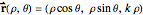 . Our intent is to calculate the geodesic curve from
  to
to  . Following the nomenclature in [2], let overscript dots indicate derivatives with respect to any general parameter
  , that is,
  .
.
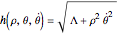
The partial derivatives on the arc-length of a curve lying on the cone are given by
 ,
,
where  .
.
Suppose a curve lying on the cone joining  and
and  is traversed along the curve
  with
with  to
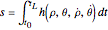
to  . The total arc-length traveling from to can be written as:
 ,
,
where  .
.
The Euler–Lagrange (EL-1,2) equations to solve the geodesic as a BVP for which the arc-length is stationary are given by
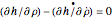 ,
,
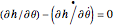 .
.
Suppose  is taken as a dependent variable and as the independent variable, that is, using in place of , the expression for
  changes to
 ,
,
 .
.
EL-1 yields a trivial solution, namely 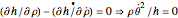 gives
gives  or
or  , which represent meridians. Meridians are geodesics for all surfaces of revolution [1, 2]. Now in EL-2,
  . Therefore,
  is a constant. Let
  , which gives
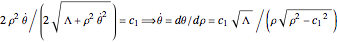 .
.
The differential equation above with the substitution  has the solution
  . By substituting the inverse for &straightpi;, we get the final equation
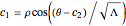 .
.
The constants  and
and  are known from the boundary conditions
  ,
,  ,
,  , and
, and  substituted.
This method can be used for any general surface of revolution, as explained in [2]. The difficulty lies in the differential equation for which was tractable for a cone. For a power law surface where  , solutions could be found using Mathematica for
  .
.
To obtain the geodesic as an IVP, The canonical geodesic (CG) equations below have been solved with , ,  , and
, and  . Here
  and primes indicate derivatives with respect to
  , the arc-length along that geodesic, that is,
  as in [2].
 ,
,
 .
.
However,  and
and  are related by
  . Therefore, choosing a single parameter
  representing the angle of the trajectory in the
  - plane at
  and setting
  and
and  , we obtain a unique geodesic about the starting point. The CG equations above can only be solved using Mathematica's built-in numerical DE solver NDSolve due to nonlinearity.
The Demonstration is a golf-like game to illustrate the concepts discussed. Two points corresponding to and  are chosen at random on a cone of given slope
  . The geodesic as a BVP is constructed for these two points. Then an initial point given by
  is chosen. By varying the angle Φ and length
  , the geodesic as an IVP is made to pass through the two points and . The two curves coincide, reinforcing the existence of a single geodesic in a small patch.
However, if one continues to play with more random points and varies , one can see that multiple geodesics can be formed using the IVP going through the points. One can also make a geodesic start and end at the same point.
This procedure resembles golf strokes constituted by and to set the trajectory of the ball moving on the surface of the cone to reach the desired end point. The key difference is that friction and gravity are absent. Indeed, it is shown in [2] that a particle with mass constrained to move on the cone's surface without friction and gravity would move along a geodesic.
Thus while length-minimizing arcs are part of one geodesic connecting two points, geodesics in general are not length-minimizing curves between two points. The Demonstration also helps you to understand geodesic parallel and polar coordinates [1].
References
[1] E. Kreyszig, Differential Geometry, New York: Dover Publications, 1991.
[2] T. J. Willmore, An Introduction to Differential Geometry, Mineola, NY: Dover Publications, 2012.
[3] G. Balmens. "Geodesics of a Torus Solved with a Method of Lagrange" from the Wolfram Demonstrations Project—A Wolfram Web Resource. demonstrations.wolfram.com/GeodesicsOfATorusSolvedWithAMethodOfLagrange.
[4] A. Slavik. "Hyperboloid Geodesics" from the Wolfram Demonstrations Project—A Wolfram Web Resource. demonstrations.wolfram.com/HyperboloidGeodesics.
[5] A. Slavik. "Cone Geodesics" from the Wolfram Demonstrations Project—A Wolfram Web Resource. demonstrations.wolfram.com/ConeGeodesics.
[6] A. Slavik. "Pseudosphere Geodesics" from the Wolfram Demonstrations Project—A Wolfram Web Resource. demonstrations.wolfram.com/PseudosphereGeodesics.
Permanent Citation
 Dupin's Indicatrix of a Torus
Sonja Gorjanc and Desana ?tambuk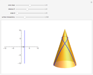 Cone Geodesics
Antonin Slavik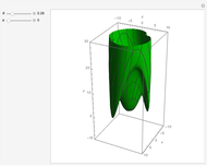 Geodesic Cone in Nil-Geometry
Benedek Schultz and János Pallagi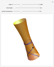 Hyperboloid Geodesics
Antonin Slavik Geodesics and Conjugate Loci on a Torus
Matthew Cherrie and Thomas Waters Geodesic Balls in the Nil-Space
Benedek Schultz, János Pallagi Conic Sections: The Double Cone
Phil Ramsden Surfaces of Revolution with Constant Gaussian Curvature
Antonin Slavik Normal Curvature at a Regular Point of a Surface
Desana ?tambuk (University of Zagreb)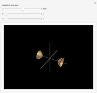 Elliptic Hyperboloid of Two Sheets
Jeff Bryant
-
 Yield under a Rigid Toroidal Indenter
Raja Kountanya -
 Shear-Angle Models for Oblique Metal Cutting
Raja Kountanya -
 Ray Tracing for Points in a Polygon
Raja Kountanya -
 Boundary and Hole Detection
Raja Kountanya -
 Component Identification and Boundary Delineation
Raja Kountanya -
 Using Eigenvalue Analysis to Rotate in 3D
Raja Kountanya -
 Chatter Stability with Orthogonal Rotation
Raja Kountanya -
 Boundary Value Problems for Cone Geodesics
Raja Kountanya