Chaotic Data: Delay Time and Embedding Dimension


Requires a Wolfram Notebook System
Interact on desktop, mobile and cloud with the free Wolfram Player or other Wolfram Language products.
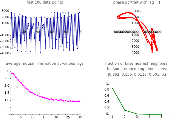
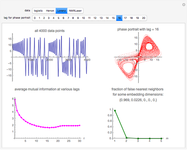
This Demonstration shows how to determine the delay time and embedding dimension for four datasets (each of length 4000). The data is derived from the logistic, Hénon and Lorenz models and NMR laser data. The delay time can be inferred from the average mutual information at various time lags: the suitable delay time is the time lag for which there is a local minimum in the average mutual information. Or, if a local minimum does not exist, the time lag at which the first substantial decrease in the average mutual information has occurred.
[more]
Contributed by: Heikki Ruskeepää (March 2017)
Open content licensed under CC BY-NC-SA
Snapshots


Details
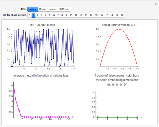
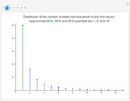
Snapshot 1: Logistic data. The phase portrait unfolds with a time lag of 1, suggesting that the delay time could be 1. The average mutual information does not have a local minimum, but the first substantial decrease stops at time lag 1, suggesting that a suitable delay time could be 1. The fraction of false nearest neighbors drops to zero for embedding dimension 1. In summary, the delay coordinates are simply  .
.
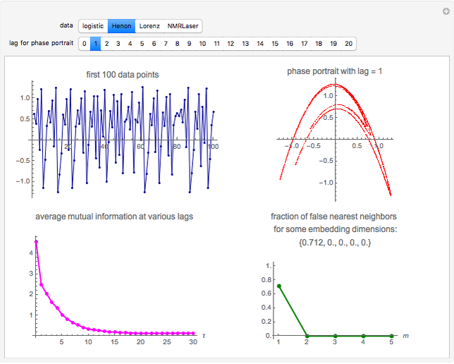
Snapshot 2: Hénon data. The phase portrait unfolds with a time lag of 1, suggesting that the delay time could be 1. The average mutual information does not have a local minimum, but the first substantial decrease stops at time lag 1, suggesting that a suitable delay time could be 1. The fraction of false nearest neighbors drops to zero for embedding dimension 2 (71.2% of nearest neighbors are false for embedding dimension 1). In summary, the delay coordinates are  .
.
Snapshot 3: Lorenz data. The phase portrait unfolds with a time lag of approximately 16, suggesting that the delay time could be 16. The average mutual information has a local minimum at a time lag of approximately 16, suggesting that a suitable delay time could be 16. The fraction of false nearest neighbors drops to zero for embedding dimension 3 (for embedding dimension 1 it is 96.9%; for embedding dimension 2 it is 2.26%). In summary, the delay coordinates are 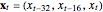 .
.
Snapshot 4: NMR laser data. The phase portrait unfolds with a time lag of 1, suggesting that the delay time could be 1. The average mutual information does not have a clear local minimum, but the first substantial decrease stops at time lag 1, suggesting that a suitable delay time could be 1. The fraction of false nearest neighbors drops to zero for embedding dimension 5 (for embedding dimensions 1, 2, 3 and 4 it is 86.2%, 13.6%, 1.18% and 0.1%, respectively). In summary, the delay coordinates are  .
.
These four settings are set as bookmarks in the "Bookmarks/Autorun" menu.
Datasets
Each of the four datasets contains 4000 values. The logistic and Hénon datasets are generated from the corresponding difference equation models. These two calculations start with a high enough precision so that even the decimal parts of the last value are all correct (for the logistic and Hénon data, we start with a precision of 2800 and 1200 digits, respectively).
The Lorenz dataset is calculated by sampling from the numerical solution of the three Lorenz differential equations. We have tried to get a high-precision numerical solution by using a working precision of 25, and accuracy and precision goals of 18 (with these settings, we need almost  steps).
For each of these three datasets, 4500 values are actually generated, but the first 500 values are dropped as transient. The NMR laser dataset was earlier available at http://people.maths.ox.ac.uk/mcsharry/lectures/ndc/ndcworkshop.shtml, but appears now to have disappeared. This dataset originally contained  values, but we only use the first 4000 values.
Phase Space Reconstruction
In phase space reconstruction, we have data in the form of a time series  ,
,  , …, and we choose a delay time
  and an embedding dimension
  to get -dimensional delay coordinates
  . In this Demonstration, we consider the estimation of the delay time and the embedding dimension.
Delay Time
There is no rigorous way to determine an optimal value for the delay time, often denoted by . In practice, the value of should be such that the values of  and
and  are sufficiently independent to be useful as coordinates in a time-delay vector but not so independent as to have no connection with each other at all. If the signal has a strong (almost) periodic component, a good first guess for the delay time is one-quarter of the period. One of the methods suggested for choosing
  is the use of mutual information. It measures the general dependence of two variables (recall that autocorrelation, well-known from time series analysis, measures the linear dependence of two variables). In this method, we calculate the average mutual information
  of the variables and for various values of :
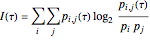 .
.
Here,  is the relative frequency of the
  bin of a histogram of the data, that is, the approximate probability that an observation is inside the bin. Similarly,
  is the approximate probability that is in the bin and is in the
  bin. The first minimum of average mutual information marks the delay time where adds maximal information to the knowledge we have from . Accordingly, it is suggested that this value of is used as the delay time in phase space reconstruction.
Embedding Dimension
A widely used method to determine is the method of false nearest neighbors. The idea is that when the embedding dimension is too small, some points of the data are very close to one another, not on the basis of the dynamics, but because the data is projected onto a too low-dimensional space. In the method of false nearest neighbors, we gradually increase the embedding dimension , and for each value of , we search for any false nearest neighbors for each point of the embedded data. This search proceeds as follows.
When we have increased to a value for which we, for the first time, essentially do no not have any more false nearest neighbors, we have identified the correct embedding dimension. For this dimension, the proportion of false nearest neighbors is either essentially zero or very small.
Related Works
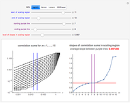
For details of analysis of chaotic data with Mathematica, see "Analysis of Chaotic Data with Mathematica" in the Related Links, in which we calculate the correlation dimension and the maximal Lyapunov exponent and also consider prediction for the four datasets.
In the other Demonstrations listed in Related Links, we estimate the correlation dimension and the maximal Lyapunov exponent.
Permanent Citation
 Chaotic Data: Correlation Dimension
Heikki Ruskeepää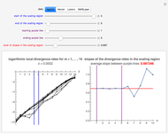 Chaotic Data: Maximal Lyapunov Exponent
Heikki Ruskeepää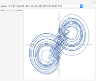 Some Time-Delay Differential Equations
Enrique Zeleny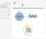 Simplest Chaotic Circuit
Bharathwaj Muthuswamy Chaotic Oscillation Circuit
Michael Schreiber Synchronization of Chaotic Attractors
Clay Gruesbeck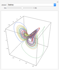 A Collection of Chaotic Attractors
Enrique Zeleny Memristor Based Chaotic System
Bharathwaj Muthuswamy (University of California, Berkeley; Milwaukee School of Engineering)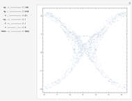 Chaotic Motion of Perturbed Pendulum
Enrique Zeleny Chaotic Itinerary but Regular Pattern
Bernard Vuilleumier
-
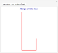
 Obtuse Random Triangles from Three Points in a Rectangle
Heikki Ruskeepää -
Chaotic Data: Maximal Lyapunov Exponent
Heikki Ruskeepää -
Chaotic Data: Correlation Dimension
Heikki Ruskeepää -
 Chaotic Data: Delay Time and Embedding Dimension
Heikki Ruskeepää -
 Method of Support Vector Regression
Heikki Ruskeepää -
 Local Regression for Country Data
Heikki Ruskeepää -
 Distribution of the Sample Range of Continuous Random Variables
Heikki Ruskeepää -
 Distribution of the Sample Range of Discrete Random Variables
Heikki Ruskeepää -
 Distributions of Discrete Order Statistics
Heikki Ruskeepää -
 Distributions of Continuous Order Statistics
Heikki Ruskeepää -
 Waiting for the Next Record
Heikki Ruskeepää -
 Distribution of Discrete Records
Heikki Ruskeepää -
 Records in Sequences of Random Variables
Heikki Ruskeepää -
 Distribution of Records
Heikki Ruskeepää -
 The Three-Tower Problem
Heikki Ruskeepää -
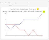 Walking Randomly Until No Shoes Are Available
Heikki Ruskeepää -
 A Reluctant Random Walk
Heikki Ruskeepää -
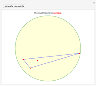 Concave Random Quadrilaterals from Four Points in a Disk
Heikki Ruskeepää -
 Obtuse Random Triangles from Three Parts of the Unit Interval
Heikki Ruskeepää -
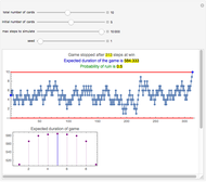
 Spin Game
Heikki Ruskeepää