Comparing Gamma and Log-Normal Distributions


Requires a Wolfram Notebook System
Interact on desktop, mobile and cloud with the free Wolfram Player or other Wolfram Language products.
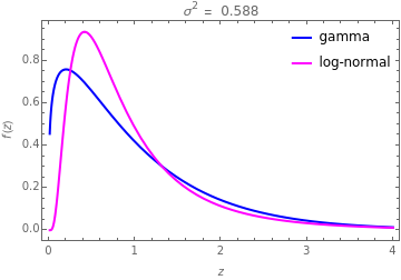
This Demonstration compares the gamma distribution  and the log-normal distribution
  . Both of these distributions are widely used for describing positively skewed data. Various distribution plots are shown as well as a table comparing the coefficients of skewness and kurtosis, denoted by
  and
and  , respectively. Plots of the probability density function (pdf) of the distributions are useful in seeing the overall shape of the distribution but other plots provide additional insights. For example, the
  plot and normal probability plot are better for showing small differences in the tails.


Contributed by: Abdelhameed El-Shaarawi, Nagham Muslim Mohammad, and Ian McLeod (August 2013)
(Department of Statistical and Actuarial Sciences, Western University)
Open content licensed under CC BY-NC-SA
Snapshots

Details
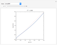
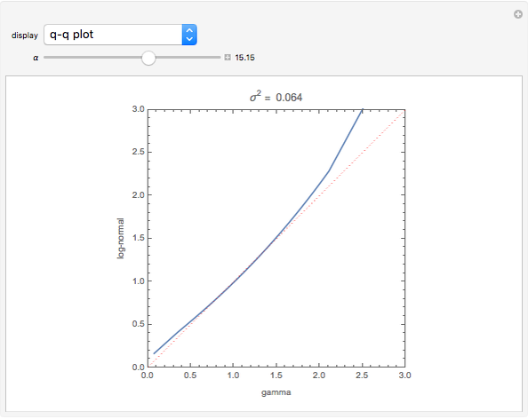
Snapshot 1. The q-q plot can be used to compare two distribution functions by plotting the quantiles of one distribution against those of another. It is the best plot to use to highlight the differences in the tails of the distributions [1]. The concave shape of the plot in the upper right quadrant indicates that gamma distribution has a slightly thicker right tail than the log-normal distribution when  .
.
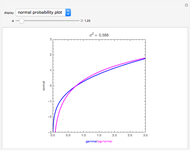
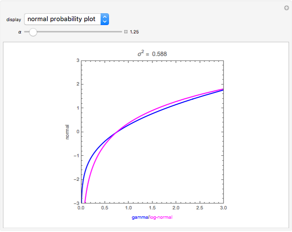
Snapshot 2: The normal probability plot displays the quantiles of the gamma/log-normal distribution versus the standard normal. From this plot we see that relative to normal, both the gamma and lognormal distributions have thicker right tails. Since the gamma and log-normal distributions are truncated at zero, outliers on the left cannot occur, so both distributions have thin left tails relative to the normal.
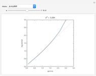
Snapshot 3: The q-q plot with  shows that the right tail of the log-normal is thicker than the gamma due to the convex curve of the q-q plot. By experimenting with various
  we found that when
  , the distributions are similar in the right tails, while for smaller values of
  , the gamma distribution has thicker right tails. As increases past 1.6, the right tail for the log-normal becomes heavier.
Snapshot 4. The p-p plot is a another parametric plot showing  , where
  is the cumulative distribution function (cdf) of the indicated distribution. The p-p plot is not as sensitive to differences in the tails of the distribution as the q-q plot, but is sometimes helpful in highlighting other differences. This type of plot is briefly discussed in [2].
Snapshot 5. The plot of the cdf also provides a visual summary that is useful for comparing distributions.
Snapshot 6. The survival function is the complement of the cdf and provides another visual comparison.
Snapshot 7. The hazard function is compared when  ; the gamma distribution has a constant failure rate, whereas the log-normal does not.
Snapshot 8. The table shows that when the coefficients of skewness and kurtosis are larger for the log-normal distribution than the gamma distribution. This is true for all values of as may be verified by experimenting with other values of or by using Mathematica symbolics to derive algebraic formulas for the skewness and kurtosis for the gamma and log-normal distributions subject to the constraints.
Reference
[1] W. S. Cleveland, Visualizing Data, Summit, NJ: Hobart Press, 1993.
[2] Wikipedia. "P-P Plot." (Aug 5, 2013) en.wikipedia.org/wiki/P-P_plot.
Permanent Citation
 Variance-Gamma Distribution
Peter Falloon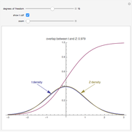 Student's t-Distribution
Chris Boucher Comparing Exact and Approximate Censored Normal Likelihoods
Ian McLeod and Nagham Muslim Mohammad The Empirical Rule for Normal Distributions
Marc Brodie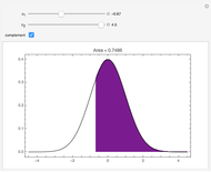 Standard Normal Distribution Areas
Ian McLeod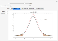 Student's t-Distribution and Its Normal Approximation
Ian McLeod Impact of Sample Size on Approximating the Normal Distribution
Paul Savory (University of Nebraska-Lincoln) Sensor Fusion with Normally Distributed Noise
Aaron Becker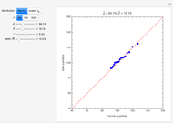 Estimating and Diagnostic Checking in Censored Normal Random Samples
Nagham Muslim Mohammad and Ian McLeod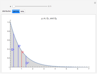 Mean, Median, and Quartiles in Skewed Distributions
Ian McLeod
-
 Rank Transform in Harmonic Regression Time Series
Ian McLeod -
 Detecting Periodicity in Short Time Series
Ian McLeod -
 Tempered Fractionally Differenced White Noise
Ian McLeod -
 Regression toward the Mean
Ian McLeod -
 Spread-Location Regression Diagnostic Check
Ian McLeod -
 Anscombe Quartet
Ian McLeod -
 Visualizing Higher-Dimensional Data with 3D Scatterplots
Ian McLeod -
 Mean, Fitted-Value, Error, and Residual in Simple Linear Regression
Ian McLeod -
Estimating and Diagnostic Checking in Censored Normal Random Samples
Ian McLeod -
 Comparing Gamma and Log-Normal Distributions
Ian McLeod -
 Monte Carlo Expectation-Maximization (EM) Algorithm
Ian McLeod -
Comparing Exact and Approximate Censored Normal Likelihoods
Ian McLeod -
 Transformation to Symmetry of Gamma Random Variables
Ian McLeod -
 Illustrating the Central Limit Theorem with Sums of Bernoulli Random Variables
Ian McLeod -
 Hidden Correlation in Regression
Ian McLeod -
 Informal Power Assessment of the Normal Probability Plot
Ian McLeod -
 Time Series for Power-Law Decay
Ian McLeod -
 Block Bootstrap for Time Series
Ian McLeod -
 Fractional Gaussian Noise
Ian McLeod -
 Plotting a Long Time Series
Ian McLeod