Distribution of the Sample Range of Discrete Random Variables


Requires a Wolfram Notebook System
Interact on desktop, mobile and cloud with the free Wolfram Player or other Wolfram Language products.
Let  , …,
, …,  be a random sample from a probability distribution. Let
  and
and  be the smallest and the largest value in the sample. The sample range
  is
is  , that is, the difference between the largest and the smallest value. The sample range is a crude measure of the variation in the sample. The Demonstration shows the distribution of the sample range, when the sample is drawn from some well-known discrete distributions.
Contributed by: Heikki Ruskeepää (June 2014)
Open content licensed under CC BY-NC-SA
Snapshots

Details
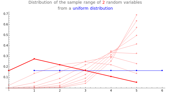
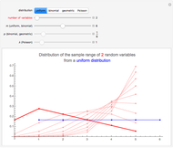
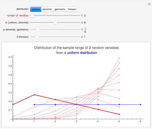
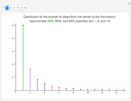
Snapshot 1: The sample is drawn from the discrete uniform distribution on the integers  ; the blue line is the probability distribution function (PDF) of the discrete uniform distribution. Each of the red curves is the PDF of a sample range: the dark red curve is the PDF of the sample range when there are only two observations. The light red curves are the PDFs of the sample range when there are 3 to 10 observations. For example, toss a die several times. With two tosses, the sample range (the difference between the results) takes on, with high probability, values from the set
  , say. Here it is less probable that the range is 0 than, say, 1; this is natural since, to get a range of zero, the results must be the same (only 6 possibilities out of 36), but to get a range of one there are more choices (10 possibilities out of 36). For three tosses, the sample range takes on, with high probability, intermediate values
  . On average, the more tosses, the larger values the sample range takes on. For example, with 10 tosses, the sample range (the difference between the largest and smallest result) takes on, with high probability, values from the set
  , say.
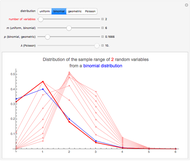
Snapshot 2: The sample is drawn from the binomial distribution: we repeat an experiment six times, each experiment being a success with probability 1/6. For example, toss a die six times and count the number of 6's; do this series of six experiments repeatedly. Repeating the six experiments two times, the sample range (the difference between the number of 6's) takes on, with high probability, values from the set  , say. Repeating the six experiments 10 times, the sample range (the difference between the largest and smallest number of 6's) takes on, with high probability, values from the set
  , say.
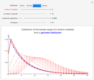
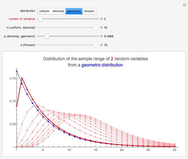
Snapshot 3: The sample is drawn from a geometric distribution with the parameter  . For example, toss a die until you get 6 for the first time. Count the number of failures, that is, the number of tosses that precede the first 6. Repeat this series of experiments several times. The distribution of the sample range for two series of experiments (the difference between the number of failures) takes on, with high probability, values from the set
  , say. For 10 series of experiments, the sample range (the difference between the largest and smallest number of failures) takes on, with high probability, values from the set
  , say.
Snapshot 4: The sample is drawn from a Poisson distribution with mean 5. For example, assume that the number of certain kinds of accidents in a given city in a day has this distribution. Consider the number of accidents in several days. For two days, the sample range (the difference between the number of accidents) takes on, with high probability, values from the set  . For 10 days, the sample range (the difference between the largest and smallest number of accidents) takes on, with high probability, values from the set
  , say.
The distributions considered in this Demonstration are (in Mathematica input):
DiscreteUniformDistribution[{1,m}], BinomialDistribution[m,p], GeometricDistribution[p], PoissonDistribution[λ].
Let the cumulative distribution function (CDF) and the probability density function (PDF) of the sample variable  be
be  and
and  , respectively. The PDF of the sample range for a sample of size
  is [1, pp. 50, 51]
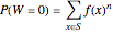 ,
,
 ,
,  .
.
where  is the support of the distribution. This formula is used to calculate the distribution of the sample range for the binomial and Poisson distributions. For the uniform and geometric distributions, we have simpler closed-form formulas in [1, pp. 51, 52].
Reference
[1] B. C. Arnold, N. Balakrishnan, and H. N. Nagaraja, A First Course in Order Statistics, Philadelphia: SIAM, 2008.
Permanent Citation
 Distribution of the Sample Range of Continuous Random Variables
Heikki Ruskeepää Distributions of Discrete Order Statistics
Heikki Ruskeepää Distribution of Discrete Records
Heikki Ruskeepää Records in Sequences of Random Variables
Heikki Ruskeepää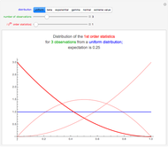 Distributions of Continuous Order Statistics
Heikki Ruskeepää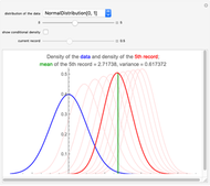 Distribution of Records
Heikki Ruskeepää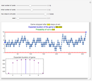 A Reluctant Random Walk
Heikki Ruskeepää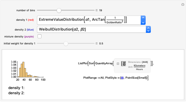 Maximum Likelihood Estimation of Ordinary and Finite Mixture Distributions
Heikki Ruskeepää and M. A. Ghorbani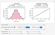 Distribution of the Means of Samples Having Random Sizes
Mark D. Normand, Joseph Horowitz, and Micha Peleg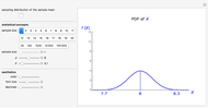 Sampling Distribution of the Sample Mean
Jim R Larkin
-
 Obtuse Random Triangles from Three Points in a Rectangle
Heikki Ruskeepää -
 Chaotic Data: Maximal Lyapunov Exponent
Heikki Ruskeepää -
 Chaotic Data: Correlation Dimension
Heikki Ruskeepää -
 Chaotic Data: Delay Time and Embedding Dimension
Heikki Ruskeepää -
 Method of Support Vector Regression
Heikki Ruskeepää -
 Local Regression for Country Data
Heikki Ruskeepää -
Distribution of the Sample Range of Continuous Random Variables
Heikki Ruskeepää -
 Distribution of the Sample Range of Discrete Random Variables
Heikki Ruskeepää -
Distributions of Discrete Order Statistics
Heikki Ruskeepää -
Distributions of Continuous Order Statistics
Heikki Ruskeepää -
 Waiting for the Next Record
Heikki Ruskeepää -
Distribution of Discrete Records
Heikki Ruskeepää -
Records in Sequences of Random Variables
Heikki Ruskeepää -
Distribution of Records
Heikki Ruskeepää -
 The Three-Tower Problem
Heikki Ruskeepää -
 Walking Randomly Until No Shoes Are Available
Heikki Ruskeepää -
A Reluctant Random Walk
Heikki Ruskeepää -
 Concave Random Quadrilaterals from Four Points in a Disk
Heikki Ruskeepää -
 Obtuse Random Triangles from Three Parts of the Unit Interval
Heikki Ruskeepää -
 Spin Game
Heikki Ruskeepää