Green's Functions with Reflection Conditions


Requires a Wolfram Notebook System
Interact on desktop, mobile and cloud with the free Wolfram Player or other Wolfram Language products.
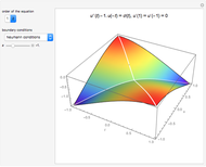
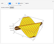
This Demonstration plots the Green’s function  for the linear differential equation with reflection of order 1,


Contributed by: Alberto Cabada, José Ángel Cid, F. Adrián F. Tojo, and Beatriz Máquez-Villamarín (December 2014)
Open content licensed under CC BY-NC-SA
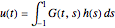
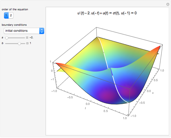
Snapshots


Details
The way to compute a Green's function for a problem with reflection is described in [1].
You can download a notebook for computing other Green's functions with reflection from [2].
References
[1] A. Cabada and F. Adrián F. Tojo, "An Algebraic Method of Obtaining the Green's Function for Some Reducible Functional Differential Equations." arxiv.org/abs/1411.5507.
[2] F. Adrián F. Tojo, A. Cabada, J. A. Cid, and B. Máquez-Villamarín, "Green's Functions with Reflection" from Wolfram Library Archive—A Wolfram Web Resource. library.wolfram.com/infocenter/MathSource/9087.
Permanent Citation
 Green's Function
Alberto Cabada, José Ángel Cid, and Beatriz Máquez-Villamarín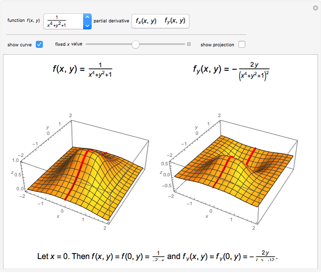 Partial Derivative Functions and Their Plots
Marc Brodie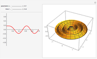 Boundary Value Problem Using Series of Bessel Functions
Stephen Wilkerson Poisson Equation on a Circular Membrane
David von Seggern (University Nevada-Reno)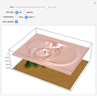 Mathematics of Tsunamis
Yu-Sung Chang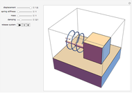 Simple Spring Mass Damping
Stephen Wilkerson (Towson University)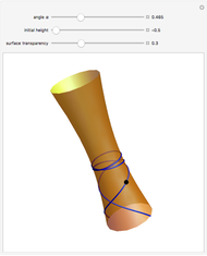 Hyperboloid Geodesics
Antonin Slavik Laplace's Equation on a Circle
David von Seggern (University of Nevada, Reno) Laplace's Equation on a Square
David von Seggern (University Nevada-Reno)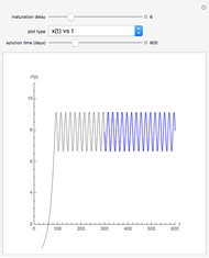 Mackey-Glass Equation
Rob Knapp