Growth Curves for a Mixture of Two Subpopulations


Requires a Wolfram Notebook System
Interact on desktop, mobile and cloud with the free Wolfram Player or other Wolfram Language products.
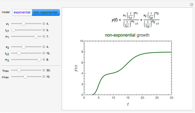
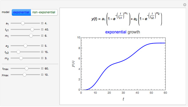
The growth curves of two-subpopulation mixtures can have shapes that are practically indistinguishable from those of a homogeneous population, but they can also have a variety of distinctly different shapes. This is shown with simulated growth curves generated with a double-stretched exponential model and a two-term non-exponential model. The Demonstration also shows how a minor change in one of the subpopulation's growth parameters can sometimes result in a major change in the shape of the mixture's growth curve.
Contributed by: Mark D. Normand, Przemyslaw Remin, and Micha Peleg (November 2014)
Open content licensed under CC BY-NC-SA
Snapshots


Details
Snapshot 1: growth curve having two inflection points generated with the non-exponential model
Snapshot 2: growth curve having two inflection points generated with the double-stretched exponential model
Snapshot 3: oddly shaped highly asymmetric growth curve generated with the double-stretched exponential model
Snapshot 4: non-sigmoid growth curve generated with the non-exponential model
Snapshot 5: typical sigmoid growth curve with a substantial lag time generated with the non-exponential model
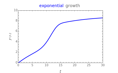
Snapshot 6: typical sigmoid growth curve with a short lag time generated with the double-stretched exponential model
Snapshot 7: typical sigmoid growth curve with a long lag time generated with the double-stretched exponential model
The growth curve of a population is frequently sigmoid or concave downward approaching an asymptotic level, primarily determined by the habitat's carrying capacity. Such curves have been described by a variety of mathematical models, which in most cases can be used interchangeably. When the population is a mixture of two subpopulations, these shapes can be maintained. However, depending on the individual subpopulation's growth parameters, the growth curve can assume different shapes that are sometimes quite atypical.
In this Demonstration, the regular and odd shapes are generated with a two-term general growth model  , where
  is either the net growth ratio
  or the logarithmic growth ratio
  , where
  and
and  are the momentary and initial sizes of the population, respectively. The first definition applies to comparatively moderate growth levels and the second to intensive growth resulting in a population rise by several orders of magnitude. According to both definitions, at
  , where
  ,
,  .
.
The chosen functions for  and
and  , whose complete formulas are displayed above the growth curve's plot, are the three-parameter stretched exponential model
  or the non-exponential model
  ), both satisfying the condition that
  . According to both models,
  , the subpopulation's asymptotic growth level,
  is a characteristic time, and
  is a steepness parameter. You can vary them and the plot's axes maxima. According to both the exponential and non-exponential models, the asymptotic growth level of the mixed population,
  , is
, is  .
.
The purpose of the Demonstration is to visualize the concept of differential population growth, not to match any experimental observation of a particular organismic or non-organismic population. Consequently, not all parameter combinations necessarily have real-life counterparts.
Permanent Citation
 Logistic Sigmoid Market Model
Michael Schreiber Uncertainties in Isothermal Microbial Growth
Mark D. Normand and Micha Peleg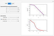 Biphasic Exponential Decay and Growth
Mark D. Normand and Micha Peleg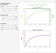 De Novo Growth Processes with Competing Mechanisms
Mark D. Normand, Maria G. Corradini, and Micha Peleg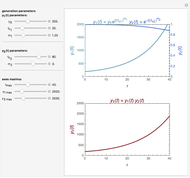 Incipient Growth Processes with Competing Mechanisms
Mark D. Normand, Maria G. Corradini, and Micha Peleg Extending the Square Root Growth Rate Model to Lethal Low Temperatures
Mark D. Normand and Micha Peleg Ratkowski's Square Root Growth Rate Model for High Temperatures
Mark D. Normand and Micha Peleg Richards Growth Curve
Georgii Alexandrov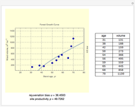 A Forest Growth Curve
Georgii Alexandrov A Model for Population Growth
Samer Hassan and Joey Espino
-
Ratkowski's Square Root Growth Rate Model for High Temperatures
Micha Peleg -
 Gordon-Taylor and Fox Equations for Glass Transition Temperature
Micha Peleg -
 Force to Overcome Vacuum Pull
Micha Peleg -
Extending the Square Root Growth Rate Model to Lethal Low Temperatures
Micha Peleg -
 Probability of Being Strange According to Paulos
Micha Peleg -
 Successive Three-Point Method for Weibullian Chemical Degradation
Micha Peleg -
 Estimating Cohesion and Tensile Strength of Compacted Powders
Micha Peleg -
 Three-Endpoints Method for Isothermal Weibullian Chemical Degradation
Micha Peleg -
 Vitamin C Loss in Foods During Heat Processing and Storage
Micha Peleg -
 Parameterizing Temperature-Viscosity Relations
Micha Peleg -
 Laplace Distribution in Fluctuating Stock Index Records
Micha Peleg -
 Weibullian Chemical Degradation
Micha Peleg -
 Simulating Ascorbic Acid Degradation
Micha Peleg -
 Additive and Multiplicative Risks
Micha Peleg -
 Endpoints Method for Predicting Chemical Degradation in Frozen Foods
Micha Peleg -
 Exponential Model for Arrhenius Activation Energy
Micha Peleg -
 Prediction of Isothermal Degradation by the Endpoints Method
Micha Peleg -
 Risk Guesstimation from Factor Ranges
Micha Peleg -
 Volatiles Formation Kinetics in Stored Fish
Micha Peleg -
 Comparison of Six Sigmoid Growth Curve Models
Micha Peleg