Kinetic Order of Degradation Reactions


Requires a Wolfram Notebook System
Interact on desktop, mobile and cloud with the free Wolfram Player or other Wolfram Language products.
Many chemical and biochemical degradation reactions follow fixed-order kinetics, including orders zero, one, or  , where need not be an integer. With the exception of first-order kinetics, which is characterized by exponential decay, the diminishing concentration versus time relationship can be described by a single formula over a range that is determined by the reactant's initial concentration,
  , the reaction’s (temperature-dependent) rate constant,
  , and the kinetic order, . This Demonstration identifies the formula’s applicability range and lets you simulate and monitor the progress of degradation reactions following any kinetic order in the range 0–2.5, with different rate constants, , and starting at different initial concentrations.
Contributed by: Mark D. Normand and Micha Peleg (July 2013)
Open content licensed under CC BY-NC-SA
Snapshots
Details
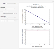
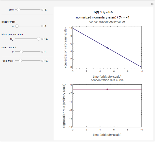
Snapshot 1: zero-order kinetics
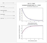
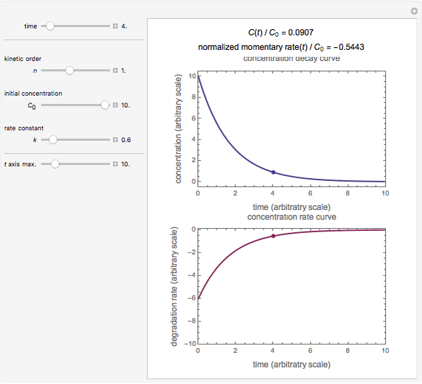
Snapshot 2: first-order kinetics
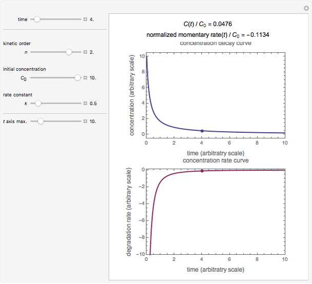
Snapshot 3: second-order kinetics
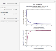
Snapshot 4: fractional-order kinetics ( )
)
Isothermal degradation of chemical reactions and biological decay processes frequently follow fixed-order kinetics with the exponent in the differential rate equation  . In this equation,
  is the concentration at time
  and is the (temperature-dependent) rate constant in the corresponding units of concentration and time. For zero-order kinetics (
 ),
),  , where is the initial concentration. For first-order kinetics (
 ),
),  , and for any other order,
 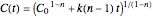 . Note that for this equation reduces to
  .
.
In an actual degradation process such as molecule disintegration, enzyme denaturation, or cell or organism mortality, neither the concentration nor density can have negative or complex values. Thus, the general equation for  -order kinetics is only applicable for , , , and combinations for which this does not happen. For , this means that the model is valid only for time
  , beyond which
  , and for , this time is
  .
.
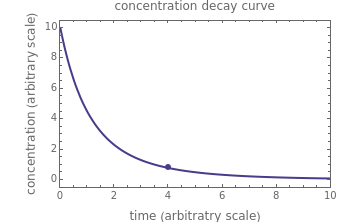
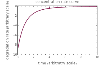
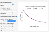
This Demonstration lets you generate degradation curves for any kinetic order in the range of 0 to 2.5 and various combinations of and by identifying the case and using the relevant formula. You can vary all three parameters , , and , as well as the actual time and process duration. The graphic display shows the concentration decay curve (top) and corresponding degradation rate versus time curve (bottom). Also shown are the numerical values of the momentary decay ratio,  , and the decay rate,
  , which correspond to the moving dots on the concentration and rate versus time plots.
The purpose of this Demonstration is to illustrate the concept of a reaction’s kinetic order. Therefore, not all possible decay rate curves represent an actual physical disintegration or degradation process.
Permanent Citation
 Fit of First-Order Kinetic Model in Degradation Processes
Mark D. Normand and Micha Peleg Extracting Fixed-Order Degradation Kinetics by the Endpoints Method
Mark D. Normand and Micha Peleg Kinetic and Thermodynamic Control of Electrophilic Addition Reactions
D. Meliga and S. Z. Lavagnino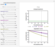 Thermal Degradation of Three Nutrients in Foods
Mark D. Normand and Micha Peleg Simulating Ascorbic Acid Degradation
Mark D. Normand and Micha Peleg Weibullian Chemical Degradation
Mark D. Normand and Micha Peleg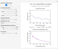 Degradation Parameters from Concentration Ratios
Mark D. Normand and Micha Peleg Prediction of Isothermal Degradation by the Endpoints Method
Mark D. Normand and Micha Peleg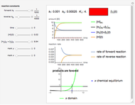 Chemical Equilibrium and Kinetics for HI Reaction
S. Z. Lavagnino and D. Meliga Successive Three-Point Method for Weibullian Chemical Degradation
Mark D. Normand and Micha Peleg
-
 Ratkowski's Square Root Growth Rate Model for High Temperatures
Micha Peleg -
 Gordon-Taylor and Fox Equations for Glass Transition Temperature
Micha Peleg -
 Force to Overcome Vacuum Pull
Micha Peleg -
 Extending the Square Root Growth Rate Model to Lethal Low Temperatures
Micha Peleg -
 Probability of Being Strange According to Paulos
Micha Peleg -
Successive Three-Point Method for Weibullian Chemical Degradation
Micha Peleg -
 Estimating Cohesion and Tensile Strength of Compacted Powders
Micha Peleg -
 Three-Endpoints Method for Isothermal Weibullian Chemical Degradation
Micha Peleg -
 Vitamin C Loss in Foods During Heat Processing and Storage
Micha Peleg -
 Parameterizing Temperature-Viscosity Relations
Micha Peleg -
 Laplace Distribution in Fluctuating Stock Index Records
Micha Peleg -
Weibullian Chemical Degradation
Micha Peleg -
Simulating Ascorbic Acid Degradation
Micha Peleg -
 Additive and Multiplicative Risks
Micha Peleg -
 Endpoints Method for Predicting Chemical Degradation in Frozen Foods
Micha Peleg -
 Exponential Model for Arrhenius Activation Energy
Micha Peleg -
Prediction of Isothermal Degradation by the Endpoints Method
Micha Peleg -
 Risk Guesstimation from Factor Ranges
Micha Peleg -
 Volatiles Formation Kinetics in Stored Fish
Micha Peleg -
 Comparison of Six Sigmoid Growth Curve Models
Micha Peleg