Parametric Density Estimation Using Polynomials and Fourier Series


Requires a Wolfram Notebook System
Interact on desktop, mobile and cloud with the free Wolfram Player or other Wolfram Language products.
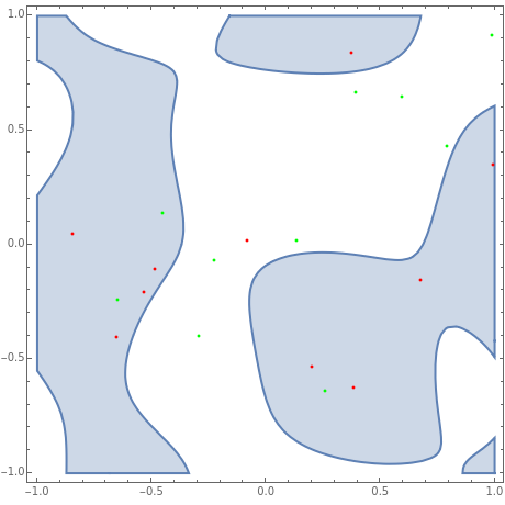
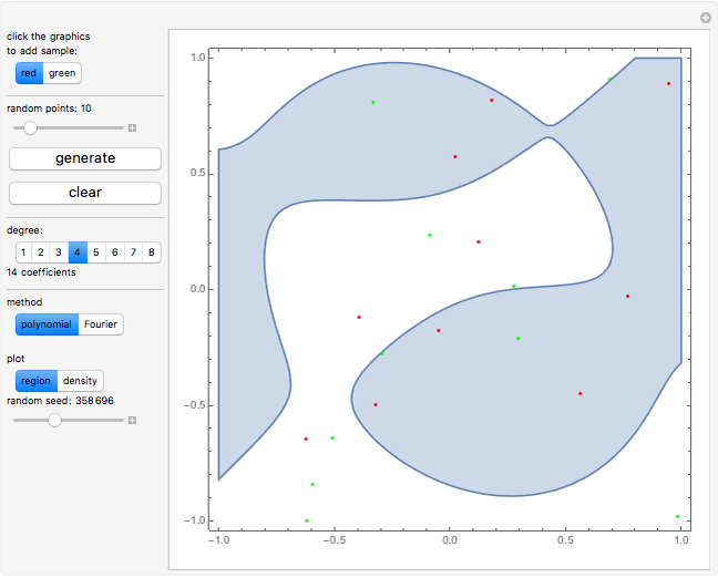
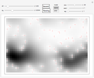
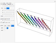
Imagine you obtain samples of two types, such as the red and green points in the graph shown here, and you would like to generalize by classifying some other points into one of these two classes. This is a basic problem in machine learning called supervised classification, with the class of each sampled point known. The standard approach is based on linear classifiers: using (hyper) planes for separation into two classes, analogous to its use in support vector machines or neural networks.
[more]
Contributed by: Jarek Duda (March 2017)
Open content licensed under CC BY-NC-SA
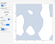
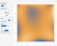
Snapshots


Details
The method used for fitting density is described in [1]. The formula was derived by smoothing the sample through convolution with a kernel, then fitting a polynomial or Fourier series to the smoothed sample. It turns out that for mean-square fitting, we can perform the limit to a zero-width kernel, giving asymptotically optimal coefficients with a very simple formula.
Specifically, assuming orthonormal bases of functions (Legendre polynomials or sines and cosines here), the linear coefficient for a given function turns out to be just the average of the function over the sample:
 ,
,
where  is the average of
  over the sample.
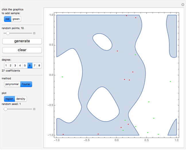
For the classification problem in this Demonstration, this density for green points was subtracted from the density for red points. Either the region of positive values (RegionPlot) or its density (DensityPlot) is then drawn.
Reference
[1] J. Duda, "Rapid Parametric Density Estimation." (Mar 14, 2017) arxiv.org/abs/1702.02144.
Permanent Citation
 Bernstein Polynomials
Yu-Sung Chang Taylor Series
Michael Ford Graphs of Taylor Polynomials
Abby Brown Polynomial Fits of Random Walks
Michael Schreiber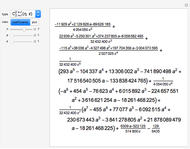 Ince Polynomials
Enrique Zeleny Taylor Polynomials
Harry Calkins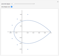 Szegö Curve
Eric Rowland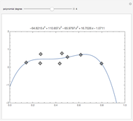 Curve Fitting
Theodore Gray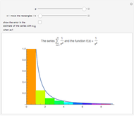 The Integral Test and Error Estimation Using p-Series
Marc Brodie (Wheeling Jesuit University)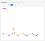 Polinomios de Taylor de las Funciones Elementales (Spanish)
Rafael Villa
-
 Parametric Density Estimation Using Polynomials and Fourier Series
Jarek Duda -
 Kepler Problem with Classical Spin-Orbit Interaction
Jarek Duda -
 Electron Conductance Models Using Maximal Entropy Random Walks
Jarek Duda -
 MU-MIMO Beamforming by Constructive Interference
Jarek Duda -
 Separation of Topological Singularities
Jarek Duda -
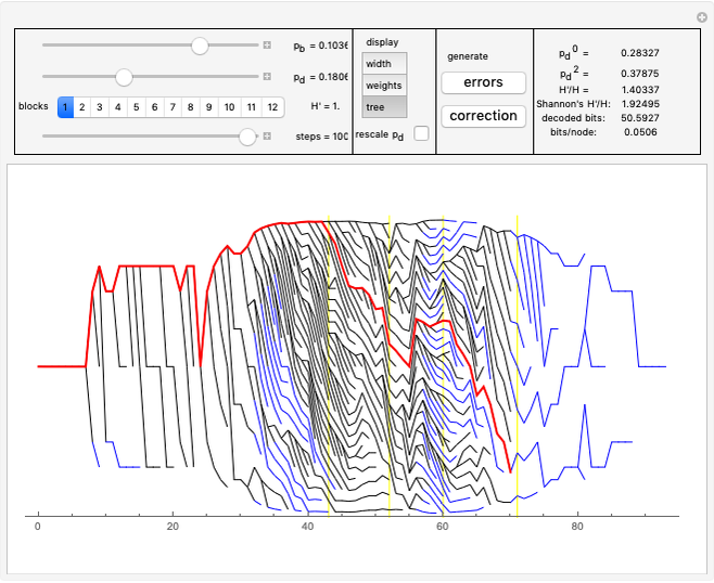 Correction Trees
Jarek Duda -
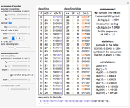 Data Compression Using Asymmetric Numeral Systems
Jarek Duda -
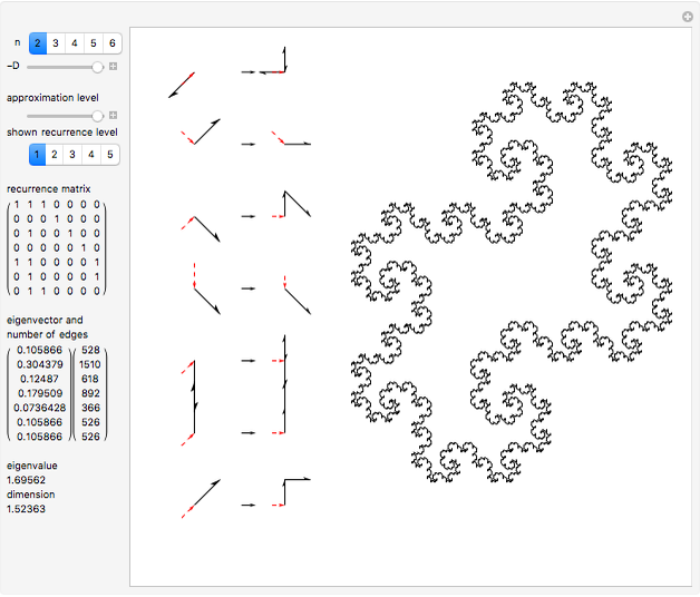 The Boundary of Periodic Iterated Function Systems
Jarek Duda -
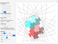 Number Systems Using a Complex Base
Jarek Duda -
 Number Systems in 3D
Jarek Duda