Pricing Put Options with the Trinomial Method


Requires a Wolfram Notebook System
Interact on desktop, mobile and cloud with the free Wolfram Player or other Wolfram Language products.
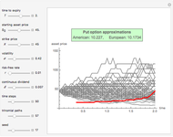
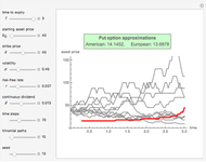
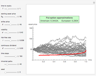
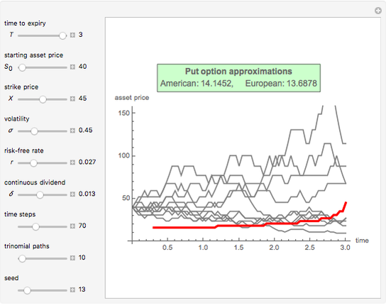
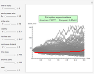
This Demonstration applies the trinomial method (also known as the "three-jump process" [2]) to approximate the value of a put option. Use the controls to set the option's parameters and the time discretization, in order to approximate the American and the European puts. The European put can be exercised only at its maturity, while the American put can be exercised at any time up to maturity. The early exercise boundary is shown with the red line; whenever the asset price drops below this boundary, the American put's intrinsic value becomes greater than its holding value, and it is optimal for the holder to exercise the option. Random trinomial paths show where the asset price is more likely to move.
Contributed by: Michail Bozoudis (July 2014)
Suggested by: Michail Boutsikas
Open content licensed under CC BY-NC-SA
Snapshots


Details
Under the trinomial method [2], the underlying asset price is modeled as a recombining tree, where at each node the price has three possible paths: an up, down, and stable, or middle, path. These values are found by multiplying the value at the current node by the appropriate factor  ,
,  , or
, or  :
:


with corresponding probabilities:


 ,
,
where  is the asset price volatility,
  is the continuous dividend yield,
  is the risk-free rate, and
  is the length of each time step in the trinomial tree (equal to the option's maturity divided by the number of time steps).
The above probabilities derive from the application of the explicit finite-difference method [3] to solve the Black–Scholes-Merton partial differential equation. The explicit finite-difference method is similar to the trinomial method, in that both provide an explicit formula for determining future states of the option process in terms of the current state. To make sure that all probabilities are in the interval (0,1), the condition  should be satisfied.
Once the trinomial lattice of all possible asset prices up to maturity has been calculated, the option value is found at each node largely as for the binomial model [1], by working backward from the final nodes to the present. The difference between the trinomial and binomial models is that the option value at each non-final node is determined based on the three, as opposed to two, later nodes and their corresponding probabilities.
The trinomial model is considered to produce more accurate results than the binomial model when fewer time steps are modeled, and is therefore used when computational speed or resources may be an issue.
References
[1] J. Cox, S. Ross, and M. Rubinstein, "Option Pricing: A Simplified Approach," Journal of Financial Economics, 7(3), 1979 pp. 229–263.
[2] P. Boyle, "Option Valuation Using a Three Jump Process," International Options Journal, 3, 1986 pp. 7–12.
[3] M. Brennan and E. Schwartz, "Finite Difference Methods and Jump Processes Arising in the Pricing of Contingent Claims: A Synthesis," The Journal of Financial and Quantitative Analysis, 13(3), 1978 pp. 461–474. doi:10.2307/2330152.
Permanent Citation
 Pricing Put Options with the Binomial Method
Michail Bozoudis Pricing Put Options with the Crank-Nicolson Method
Michail Bozoudis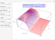 Pricing Put Options with the Explicit Finite-Difference Method
Michail Bozoudis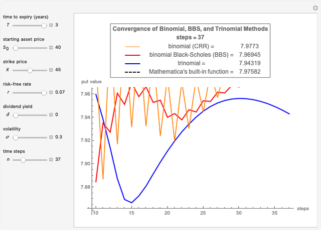 Convergence of Binomial, Binomial Black-Scholes, and Trinomial Option Pricing Methods
Michail Bozoudis Kim's Method for Pricing American Options
Michail Bozoudis A Recursive Integration Method for Options Pricing
Michail Bozoudis Kim's Method with Nonuniform Time Grid for Pricing American Options
Michail Bozoudis Adaptive Mesh Relocation-Refinement (AMrR) on Kim's Method for Options Pricing
Michail Bozoudis Pricing American Options with the Lower-Upper Bound Approximation (LUBA) Method
Michail Bozoudis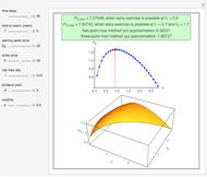 Pricing American Options with the Two- and Three-Point Maximum Methods
Michail Bozoudis
-
 Fitting Times-to-Failure to a Weibull Distribution
Michail Bozoudis -
 A Canonical Optimal Stopping Problem for American Options
Michail Bozoudis -
A Recursive Integration Method for Options Pricing
Michail Bozoudis -
Adaptive Mesh Relocation-Refinement (AMrR) on Kim's Method for Options Pricing
Michail Bozoudis -
Kim's Method with Nonuniform Time Grid for Pricing American Options
Michail Bozoudis -
 Geometric Brownian Motion with Nonuniform Time Grid
Michail Bozoudis -
Kim's Method for Pricing American Options
Michail Bozoudis -
 Simultaneous Confidence Interval for the Weibull Parameters
Michail Bozoudis -
 Binomial Black-Scholes with Richardson Extrapolation (BBSR) Method
Michail Bozoudis -
Pricing American Options with the Lower-Upper Bound Approximation (LUBA) Method
Michail Bozoudis -
 American Options on Assets with Dividends Near Expiry
Michail Bozoudis -
 Hold-or-Exercise for an American Put Option
Michail Bozoudis -
 American Capped Call Options with Exponential Cap
Michail Bozoudis -
 American Capped Call Options with Constant Cap
Michail Bozoudis -
Pricing Put Options with the Crank-Nicolson Method
Michail Bozoudis -
 Pricing Put Options with the Implicit Finite-Difference Method
Michail Bozoudis -
 Estimating a Distribution Function Subject to a Stochastic Order Restriction
Michail Bozoudis -
 Maximizing a Bermudan Put with a Single Early-Exercise Temporal Point
Michail Bozoudis -
 Fitting Data to a Lognormal Distribution
Michail Bozoudis -
 SARIMA Process Forecasting Model
Michail Bozoudis