Simulating the Branching Process

Requires a Wolfram Notebook System
Interact on desktop, mobile and cloud with the free Wolfram Player or other Wolfram Language products.
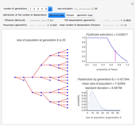
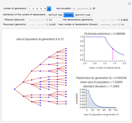
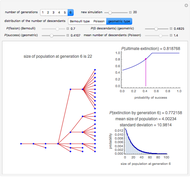
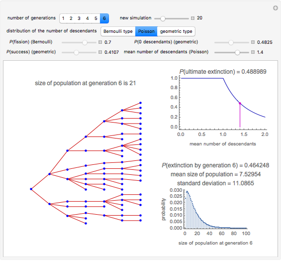
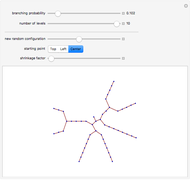
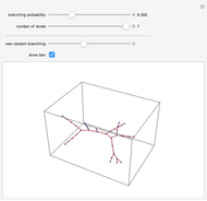
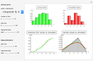
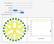
This Demonstration shows up to six simulated generations of a branching process. The distribution of the number of descendants of each member of the population can be either a Bernoulli type distribution, the Poisson distribution, or a geometric type distribution; the parameters of these distributions can be set with sliders. From the three figures, the left one shows the simulated branching process, the upper-right one shows the probability of ultimate extinction as a function of a parameter of the distribution, and the lower-right one shows the probabilities of the size of the population at the selected generation.
Contributed by: Heikki Ruskeepää (March 2013)
Based on a program by Stephen Wolfram
Open content licensed under CC BY-NC-SA
Snapshots
Details
Snapshot 1: The number of descendants has a Bernoulli distribution with the probability of fission as 0.7. At generation 6, the size of the simulated population happens to be 20. The probability of ultimate extinction is 0.429 while the probability of extinction by generation 6 is somewhat smaller, 0.421. The mean size of the population at generation 6 is 7.53 and the most common positive population size is 8. Population sizes larger than, say, 40 have very small probabilities. At generation 6, the maximum size of the population is  . Only even population sizes are possible.
Snapshot 2: The number of descendants has a Poisson distribution with the mean number of descendants as 1.4. At generation 6, the size of the simulated population happens to be 25. The probability of ultimate extinction is 0.489 while the probability of extinction by generation 6 is somewhat smaller, 0.464. The mean size of the population at generation 6 is 7.53 and the most common positive population size is 3. Population sizes larger than, say, 60 have very small probabilities at generation 6. The size of the population does not have any finite upper bound.
Snapshot 3: The number of descendants has a geometric distribution with the probability of zero descendants as 0.4825 and the probability of success as 0.4107. At generation 6, the size of the simulated population happens to be 22. The probability of ultimate extinction is 0.819 while the probability of extinction by generation 6 is somewhat smaller, 0.772. The mean size of the population at generation 6 is 4.00 and the most common positive population size is 1. Population sizes larger than, say, 80 have very small probabilities at generation 6. The size of the population does, in principle, not have any finite upper bound (although to speed up the Demonstration, we have defined that the maximum number of descendants of each individual is 20).
In a branching process, a population evolves in generations, starting from a single individual (this is the zeroth generation). Each individual of the current generation produces, independently of other individuals, a number of descendants according to a known probability distribution. The descendants constitute the next generation. We are interested in the size of the successive generations.
Let  be the random variable that gives the number of descendants of each individual. In the Demonstration, we consider three distributions of
  : a Bernoulli distribution, the Poisson distribution, and a geometric distribution.
1. In the Bernoulli type distribution,  gets either the value 0 or the value 2 with probabilities
  and
and  , respectively. This distribution may be useful in describing the fission of atoms in nuclear chain reactions; see [2, p. 294], [3, Problem 21]. This is the type of branching process considered by Stephen Wolfram in his Demonstration. In our Demonstration, we have used his ingenious code of simulating and plotting a branching process.
2. In the Poisson distribution,  gets the value
  with probability
  ,
,  , where
  is the mean number of descendants. This model may be useful in describing, for example, some problems in genes and mutations [2, p. 295].
3. In the geometric distribution,  gets the value 0 with probability
  and a value
  ,
,  , with probability
  . This distribution has been used in describing the survival of family names [2, p. 294], [3, Problem 21]. Only male descendants are taken into account. Thus,
  is the probability that any newborn boy will himself father
  boys. A. Lotka has shown in the 1930s that, at least in America, good estimates of the parameters of the geometric type distribution are
  and
and  (these are the initial values of the two parameters in the Demonstration).
Let  and
and  be the mean and variance of
  . Let
. Let  be the size of the
  generation. It can be shown that
  . Thus, if
  , the expected size of the population approaches zero, and if
  , the size of the population is expected to explode. Thus, the population will essentially either ultimately be extinct or grow without bounds. If
  , then
  ; otherwise
  .
.
Let  be the probability generating function of
  , that is,
  . Let
. Let  be the probability of ultimate extinction of the population. It can be shown that
  is the smallest non-negative solution of the equation
  . Further, we know that
  if
if  , and
, and  if
if  . For example, in the Bernoulli type distribution,
  so that
  if
if  . In the Poisson distribution,
  , so that
  if
if  . In the geometric type distribution,
  so that
  if
if  .
.
Let  be the probability generating function of
  . It can be shown that this generating function can be computed from the recursive formulas
  ,
,  ,
,  . After calculating
  , we get the probabilities of the size of the
  generation from the coefficients of the powers of
  in the power series expansion of
  . In particular, the first coefficient (the constant term) is the probability of zero individuals (meaning extinction). Note that in the lower-right figure we only show the probabilities of the population sizes 1, 2, 3, …, while the probability of size 0 is given in the plot label (this method was used because the probability of size 0 is often very much larger than the other probabilities; by dropping this probability from the plot, we can see the other probabilities more clearly). Note also that we only show probabilities of population sizes at most up to size 100.
The Demonstration was inspired by problem 21 in [3]. For more about the branching process, see, for example, [1] and [2]. See also "Branching Process" in Wikipedia.
References
[1] N. T. J. Bailey, The Elements of Stochastic Processes: With Applications to the Natural Sciences, New York: Wiley, 1964.
[2] W. Feller, An Introduction to Probability Theory and Its Applications, Vol. I, 3rd ed., New York: Wiley, 1968.
[3] P. J. Nahin, Digital Dice: Computational Solutions to Practical Probability Problems, Princeton, NJ: Princeton University Press, 2008.
Permanent Citation


