Steady-State Heat Transfer through a Composite Plane Wall


Requires a Wolfram Notebook System
Interact on desktop, mobile and cloud with the free Wolfram Player or other Wolfram Language products.
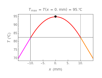
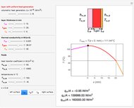
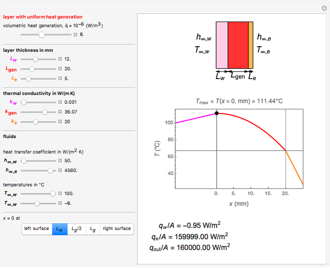
This Demonstration calculates the temperature profile across a composite plane wall. The wall is exposed to convection on both the right and left sides. The central layer has uniform volumetric heat generation. The parameters correspond to thickness and thermal conductivity for each of the three layers, internal heat generation for the central layer, and temperature and convective heat transfer coefficients for the fluids in contact with the wall surfaces on each side. The top graphic displays the nomenclature used for each layer (notice the color coding). The location and value of the maximum temperature within the layer with heat generation is displayed on the top of the plot (only when heat generation is larger than zero). The heat fluxes  at each interface between fluid and wall are described at the bottom, followed by the rate of energy per surface area that exits the wall. There are five choices for the
  axis origin: the left surface of the wall, the interface between the first two solid layers
  , the center of the layer with heat generation
  , the interface between the second and third wall
  , or the right surface of the wall.
Contributed by: Cibele V. Falkenberg (February 2016)
Open content licensed under CC BY-NC-SA
Snapshots


Details
Snapshot 1: Without any heat being generated, the temperature profile is linear in each layer (with the slope dependent on the thermal conductivity). The heat flux across the wall is constant, and is driven by the temperature difference between the fluids. You can shift the origin of the plot using the buttons at the bottom of the controls. The directionality for the heat fluxes is consistent with the axis in the plot.
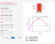
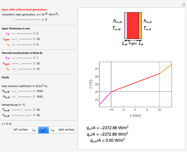
Snapshot 2: The location of the maximum temperature and fraction of the heat being transferred to each side depends on the resistances for convection and conduction on each side.
Snapshot 3: By significantly increasing the resistances on one side (left), the location of the maximum temperature also shifts toward the same side of the wall, approaching the limit of the adiabatic boundary condition. As a consequence, most of the heat generated in the volume must exit through the opposite surface.
In a steady state, the rate of energy generated within the wall (the product between  and the volume of the central layer
  ) equals the sum of the heat transfer rates leaving each side of the wall. Because the vector for the heat flux follows the direction of the axis in the plot (positive from left to right), the heat transfer rate leaving the left surface is equal to
  . The heat fluxes are described as
  , where
  is the area on each side of the wall (
 plane).
Reference
[1] T. L. Bergman, A. S. Levine, F. P. Incropera, and D. P. Dewitt, Fundamentals of Heat and Mass Transfer, 7th ed., New York: Wiley, 2011.
Permanent Citation
 Steady-State Heat Transfer through an Insulated Wall
Mark D. Normand and Micha Peleg Radiation Heat Transfer Coefficient for a Gray Surface
Cibele V. Falkenberg Steady-State 1D Conduction through a Composite Wall
Sara McCaslin and Fredericka Brown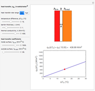 Heat Transfer in a Heat Exchanger
Mark D. Normand, Maria G. Corradini, and Micha Peleg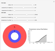 Steady-State Temperature Profile of Two-Layer Pipe
Fredericka Brown and Sara McCaslin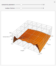 Heat Transfer along a Rod
Stephen Wilkerson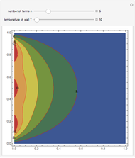 Gibbs Phenomenon in Laplace's Equation for Heat Transfer
Stephen Wilkerson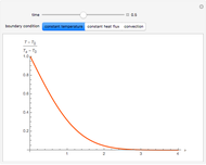 Heat Diffusion in a Semi-Infinite Region
Brian Vick Experiment on Heat Conduction
Enrique Zeleny Periodic Heat Kernel
William O. Bray