Wolfram Demonstrations Project

This Demonstration estimates the theoretical spread of a microbe's logarithmic survival ratios after isothermal heat treatment, resulting from uncertainties in its heat-resistance parameters. It is based on the assumption that the survival pattern follows the Weibullian–Log Logistic (WeLL) model with a temperature-independent shape factor. The organism or spore's three heat resistance parameters are:

, which accounts for its semi-logarithmic survival curve's concavity,

, the temperature that marks the onset of lethality, and

, t

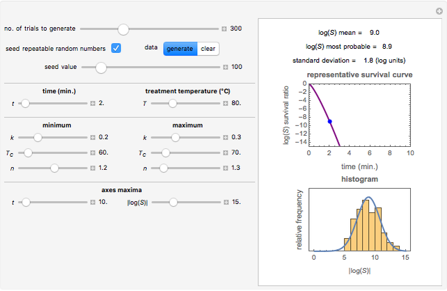
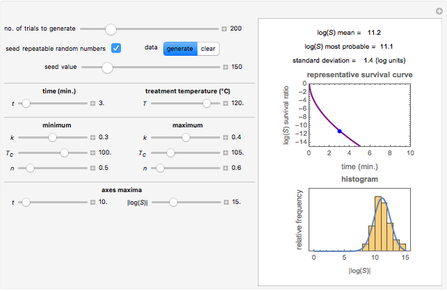
he inactivation rate rise with temperature in the lethal region. All are entered as the lower and upper limits of their plausible ranges. Monte Carlo simulations generate numerous hypothetical survival ratios with random parameter values within these ranges, whose mean and standard deviation are calculated and displayed, together with a representative survival curve and the ratios' histogram for the chosen temperature and heat-treatment duration.

Contributed by: Mark D. Normand and Micha Peleg

Slider Zoom
Automatic Animation

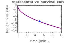
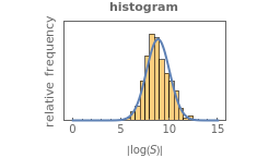
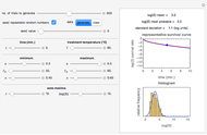
Snapshot 1: survival curve of a hypothetical pathogen having upward concavity exposed to a heat treatment and the corresponding histogram of its survival ratios

Snapshot 2: like snapshot 1 but with downward concavity

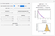
Snapshot 3: survival curve of hypothetical heat resistant Clostridium spores having upward concavity exposed to a 120 °C heat treatment and the corresponding histogram of its survival ratios

Snapshot 4: like snapshot 3 but with Bacillus spores having downward concavity

The isothermal survival curves of viruses, bacterial, yeast, or mold cells, and bacterial spores are commonly presented as plots of the logarithmic survival ratio

versus time, where

being the number of survivors after time

at a given temperature

and

their initial number. For many microorganisms [1, 2], the survival curve can be described by the Weibullian model

, where

a "rate parameter" and

a concavity index. When

, the semi-logarithmic survival has upward concavity. When

, it has downward concavity, and when

, it is linear ("first-order kinetics"). For many microbes,

has very weak temperature dependence and can be assumed constant,

, [1, 2]. The rate parameter's temperature dependence can frequently be described by the log logistic model,

, where

marks the onset of lethality and

is approximately the slope of

versus

. Incorporating this

expression in the inactivation equation produces the Weibull–Log Logistic (WeLL) survival model whose parameters are

, and

Experimental determination of microbial survival curves is hampered by technical and logistic considerations and therefore replications are frequently kept at a minimum. The occasional need to use a surrogate medium in place of the food itself and the difficulty in determining contributions of the come-up and cooling stages add to the uncertainty concerning the magnitude of experimentally determined survival parameters. Therefore, it would be more appropriate that they be treated not as single values but as the lower and upper limits of their plausible ranges.

In this Demonstration, you can enter the time

, temperature

, and the lower and upper limits of the WeLL model's survival parameters

, and

with sliders and also choose the number of Monte Carlo simulation trials. Clicking the "seed repeatable random numbers" checkbox lets you reproduce the random simulations from the same seed value. The program then generates the chosen number of simulations with random combinations of the survival parameters, assumed to be uniformly distributed within their respective ranges ("maximum ignorance") and calculates the corresponding logarithmic survival ratio using the WeLL model's equation. These ratios' mean,

, is considered the best estimate and their standard deviation,

, is the measure of the spread. A plot of the generated ratios' histogram is displayed with a superimposed PDF plot of the normal (Gaussian) distribution having the same

and

(the method of moments). In order to produce new random trial data with exactly the same parameter settings, first click the "clear" button, then click the "generate" setter.

Above the histogram, a representative complete survival curve is drawn on which the chosen time is shown as a blue dot that you can drag. You can also vary this plot's coordinate scales,

and

with sliders. The displayed representative survival curve is calculated using the WeLL model's equation with the parameters assigned the mean values of their entered lower and upper limits. The corresponding survival ratio, which is close but not identical to that calculated by the Monte Carlo simulations, is also shown for comparison above the two plots.

All the

labels on the plots refer to base-10 logarithms, as is customary in food microbiology. Not all possible control settings produce realistic survival curves.

References

[1] M. Peleg, Advanced Quantitative Microbiology for Food and Biosystems: Models for Predicting Growth and Inactivation, Boca Raton, FL: CRC Press, 2006.

[2] M. A. J. S. von Boekel, Kinetic Modeling of Reactions in Foods, Boca Raton, FL: CRC Press, 2008.

[3] M. G. Corradini, M. D. Normand, and M. Peleg, "Non-Linear Growth and Decay Kinetics—Principles and Potential Food Applications," in Food Engineering: Integrated Approaches (G. F. Gutiérrez-Lopez, G. V. Barbosa-Cánovas, J. Welti-Chanes, and E. Parada Arias, eds.), New York: Springer, 2008, pp. 47–71.